At this stage of inquiry, I moved to the business side of things to learn more about Excel as a tool for small business accounting; in this case, tracking and allocating funds earned from a private lesson business as a music teacher. Below is a video by Amber Reed, a string teacher who uploads advice for running studios under the channel name Violin Viola Masterclass. It’s a recording of a livestream that goes over the basics of the basics of tracking lessons and budgeting your gross income.
The system Reed lays out is very simple: Record how many lessons you expect to get, adjust for how many you did get, and write out how much you were paid for those lessons, separating the data by student and recording monthly. Next, start with your gross income and move 35% to your business savings account, take off 10% for you personal savings account, and take off another 10% to split between your personal and business chequing accounts. For my Excel integration, I decided to build out and automate this system as an Excel workbook.
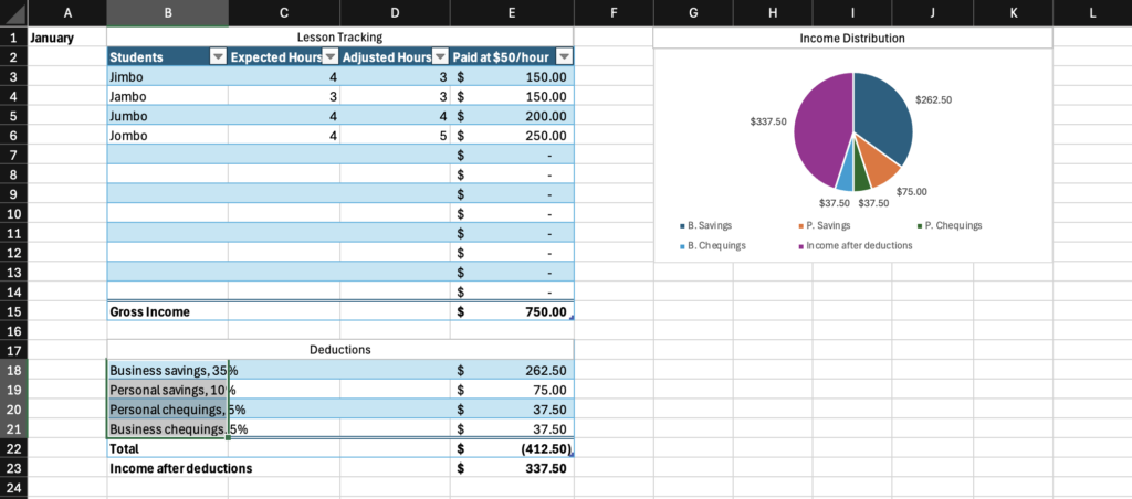
Above, you can see the January page for the tracking system and download the workbook yourself should you have the need to track a similar activity or adjust the template as you see fit. The workbook is set up for 12 months along with a full-year summary page totalling gross income and the amounts expected to be recieved in each account over the time period. In Reed’s video, she applies her percentages to a running total, pulling from a smaller number for each step, resulting in a total deduction of approximately 52%. This seems to me to be an unecessary complication of the process, and, based on the paper she shows, the system is apparently intended to save 55% of the total income anyway, so I opted to apply the percentages to the total gross income at each step, both to simplify things, and because setting aside another 3% never hurt anyone. This is hardly a comprehensive budget system, but it offers the beginning of one, and the figures it calculates can be used for input into a larger budgeting system in another template or platform.
Everything after the expected and adjusted hours in the workbook is completely automated, with the adjusted hours column feeding into the Paid column, whose total is divied up with SUM fuctions in the Deductions section, which in turn feeds into the chart and the yearly summary. I’ll note here an example of the many small conveniences of Excel that really do add up: once I input the SUM function into the first cell in the Paid column feeding from the Adjusted Hours column, I simply drag the bottom right corner to the bottom of the table and Excel will apply it to the whole thing. Copying and pasting also automatically fixes the SUM function to apply to the cell in the same source relative to the new location, so this would also have worked.
As for using the template, that first link between the Adjusted Hours column and the Paid column is the one I would most readily expect to be broken. One is rarely paid at the same time one records the adjustment, and there are myriad circumstances where your pay won’t line up perfectly with your expected rate for whatever reason. Simply selecting the cells in the column and hitting backspace will delete the SUM function and allow manual input.
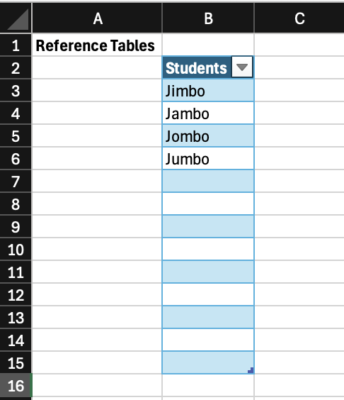
The Student column is set to a drop-down menu restricting input to the list of students found in the reference tables sheet. I don’t currently have a studio, so I’m using my example squad of Jimbo Jambo Jombo and Jumbo’s first 2 months of lessons. You can change the list of students by changing the names in the Students reference table.
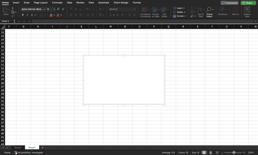
Now is about the time I start complaining, if I have come to understand my Excel Inquiry Rhythm correctly. I’ve gotten enough Excel experience that most things went well enough with the setup this time around. I did have an issue where upon moving a table, it forgot that it was a table and ruined the cell formatting, making all the backgrounds the same colour instead of the usual row by row alternation and not responding to the templates in the Table menu. I haven’t been able to recreate the glitch authentically, but it looked something like this:
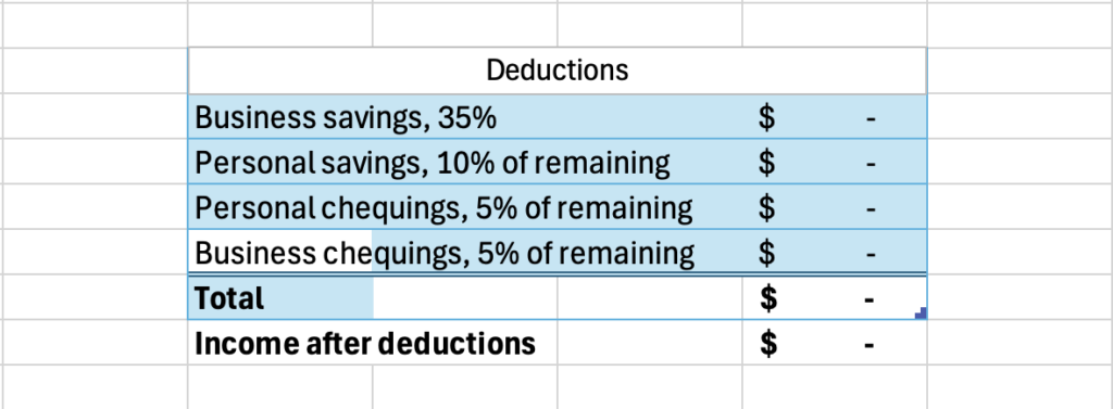
All one needs to do to fix this is select the whole table, go to the Home tab > cell styles, and select normal.
Another issue arose in the building of the “Gross income from lessons” row of the yearly summary.
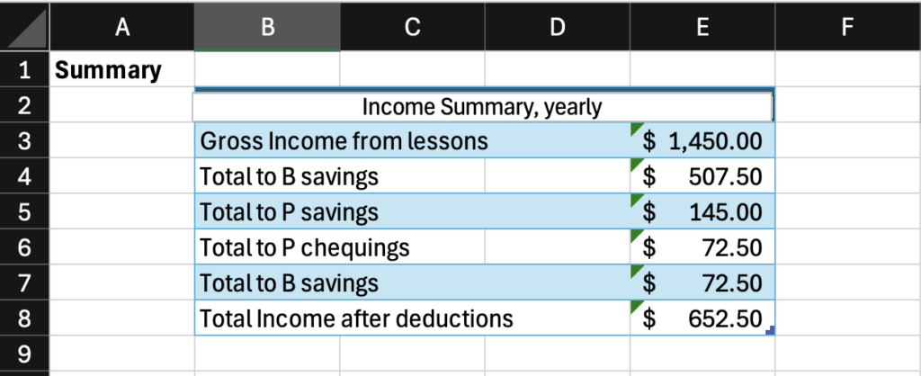
When you input a SUM function, after typing =SUM(, you can choose to either type in the cells or cell range or select the ranges you want to feed from with your mouse. I first opted to use the mouse to make my SUM function, but this will produce the following equation:
=SUM(Table1[[#Totals],[Paid at $50/hour]]+Table112[[#Totals],[Paid at $50/hour]]+Table11214[[#Totals],[Paid at $50/hour]]+Table1121416[[#Totals],[Paid at $50/hour]]+Table112141618[[#Totals],[Paid at $50/hour]]+Table11214161820[[#Totals],[Paid at $50/hour]]+Table1121416182022[[#Totals],[Paid at $50/hour]]+Table112141618202224[[#Totals],[Paid at $50/hour]]+Table11214161820222426[[#Totals],[Paid at $50/hour]]+Table1121416182022242628[[#Totals],[Paid at $50/hour]]+Table112141618202224262830[[#Totals],[Paid at $50/hour]]+Table11214161820222426283032[[#Totals],[Paid at $50/hour]])
This version does work, but when I first finished doing this, I found that I was getting the completely wrong number from the function. With a SUM this dense and enormous, there was no way I was figuring out where my error was. At this point, I had already completed the totals for the other rows with the mouse clicking method, which gave me much more manageable SUM functions of the following style:
=SUM(January!E15+February!E15+March!E15+April!E15+May!E15+June!E15+July!E15+August!E15+September!E15+October!E15+ November!E15+December!E15)
Seen above is a SUM function identical to the original, but referencing cells containing a total instead of referencing totals of columns. It’s a nitpicky sort of difference to describe, but it looks far more straightforward in the cell and is much easier to troubleshoot with. My advice here is to avoid clicking to select totals from tables when building longer SUM functions and either writing out the sheet titles, or clicking to select different cells of the same column from each sheet and then switching out the row to the correct number after the fact. There is also a chance that there is an easier way to reference the same cell on multiple sheets than inputting each one in a SUM function with a plus sign, but I don’t know how to google that and I haven’t stumbled across it yet.
The real bugbear of this operation was the pie chart. Now seems like as good a time as ever for a questionably necessary tangent about video games. A short clip from the below video by Arin Hanson is relevant here, from 00:19-1:14. The series this comes from has found its way into game design classrooms over the years, but was created informally for entertainment purposes, so the program contains coarse language, mostly outside of this clip, but viewer discretion advised.
The shift that Hanson describes in videogames, moving from programs that needed manuals to explain them, like traditional games, toward programs that could be learned intuitively over the course of interacting with them, like Mega-Man and it’s ilk, is not unique, but is in fact the path taken by essentially all digital products as they mature and reach wider audiences. No one really expects you to learn how to use something like Google Docs, it is expected that a person can do what they need to do in that program without a tutorial, relying on a user interface that draws one’s attention to key features using a logical menu system that makes it easy to find options you need.
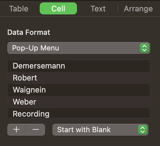
Excel is an example of a program that has rejected this trend. Recall the difference between the dropdown menus and pop-up menus in Excel and Apple Numbers, respectively. In Numbers, you always change how data is represented or input in a cell using the Data Format menu on the right of the screen, and when you select Pop-Up Menu from the Data Format options, the box to write in the list of items you want in your menu is right there in the same spot.
Contrast this to the dropdown menus in Excel, where you need to write down your list of options somewhere in the workbook first, then select the cells you want to have the dropdown menu, go to the Data tab at the top of the screen, find the small Data Validation button placed between “Text to Columns” and “What-if Analysis”, select “list” under the “Allow” subheading, then type in or select with your mouse the range of cells containing the reference list you made earlier. In this situation, Apple Numbers is the clear Mega-Man to Excel’s Godzilla for the Gameboy.
Returning to the pie chart, when I clicked the button to insert it into my sheet, this is what I saw.
Excel had given me a deck of cards and told me to figure out how to play Solitaire.
This is a slight exaggeration. I was able to figure out that “Chart Design” probably let me design the chart and that “select data” was probably going to let me select the data, so I wasn’t completely lost.
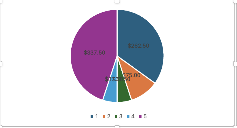
Those first steps brought me here, with an obviously unreadable mess. There was also originally a title for the graph that I removed and am not so committed to this reanactment that I will add back in, but I will say to be careful when hitting backspace around a chart in Excel, because if you have the wrong element selected it will delete the whole thing in a way that doesn’t let undo commands bring it back, so you’ll need to start over. Backspace is also how you get rid of the title on the chart.
First, I wanted to get my numbers outside of the circle, which you do by selecting Add Chart Element > Data Labels > Outside End. I had to find this on the Microsoft support page, since I don’t know how moving the labels from one place to another could be considered adding an element, so I didn’t think to look there.
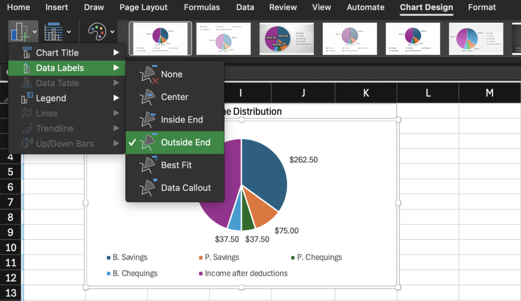
Next, I wanted to add descriptive labels to the legend instead of numbers, which you can see completed in the above image. I first tried selecting the labels on the chart and typing in the descriptions that I wanted. Like an absolute Chump. If you think that would work you have learned nothing about Excel. You have to make a reference table somewhere else, of course! You then need to go back to the Data Selection menu and type the range of cells containing the reference table into the “Horizontal (Category) axis labels” box, which I suppose would have registered less like word salad to me if the graph I was working with had axes that one could describe as horizontal, but it would be too much to expect of the trillion dollar company to have menus that adapt to the type of graph you’re working with.
The program is also quite picky about the reference table and data selection source. All items in each category must be in the same column, though they don’t need to be in adjacent rows. If your data and reference table are on the same sheet, they must be placed parallel to eachother, with each label in the same row as it’s datapoint. If either of these rules are broken, the chart will claim that the data is too complex and will display nothing. I have only been able to determine these rules through trial and error, and I may be incorrect, which has me feeling like I’m sharing Excel folklore about how if you burn a goats foot on the right day the data rains will come. Currently, all of the monthly charts after February show “The Chart Data Range is too complex to be displayed” when I open the “Select Data” menu, but they still display the data they are supposed to when it is input. Here I am following the age-old coding principal of not fixing what probably isn’t broken.

I also noticed that on the legend pictured above, the dark blue and green colour indicators corresponding to B. Savings and P. Chequings respectively were kind of difficult to separate, so I wanted to change out one of the colours. Apparently, however, you can’t customize the colours of graphs in Excel for MacOS; you only have a preset of “colourful” options, most of which use all the same colours just in different orders, or “monochromatic” options, which use gradients and make it basically impossible to tell which label corresponds to what. Earlier, I was in a menu that had a completely different set of options including making the slices hollow or all only one colour, which makes the legend entirely pointless, but I can’t even find that menu upon returning to checl. This colour restriction seems like a gap in accessibility to me, and the questionable presets and inability to change them is another example of what I can only see as frustrating laziness on the Microsoft development teams.
Excel is a program designed to be learned by reading pages and pages of manuals and watching hours and hours of tutorials. I whine and complain, of course, but really it is not such a bad thing that Excel is not a video game. Things don’t need to be simple and straightforward to be functional, and most things in real life designed to meet a particularly specific need expect a person to be willing and able to dedicate the time and energy into figuring them out. Excel is just one of these things. At the end of the day, my tracker is still functional and helpful, and I was able to attain the skills to build it over the course of a relatively short deep dive. I still think they can try a little harder on the design side though.